Fast Fourier transform
Instructions
Use
Example
Principle
The fas
Fourier transform is a tool very much used in the signal processing
domain. So that it is relatively fast, it is necessary that it is
adapted to the kind of processor which must carry out it. I thus made
of it a version optimized for calculations of integers and using
trigonometrical functions SIN and COS presented in the corresponding page.
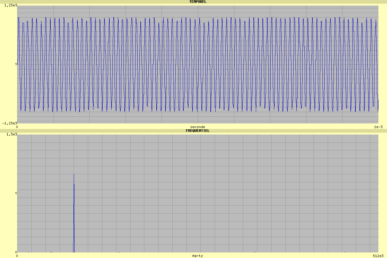
To have the results which one can obtain, I used the curves displaying application which requires the use of numbers in floating decimal point 64 bits right before posting.
Here for example the Fourier transform of a 2 KHz sinusoidal wave sampled with 512 Khz during 1 ms:


Instructions
ln(nbp)/ln(2) is corresponding to the logarithm in base 2 of the dots number (example: 10 for nbp=1024)
@temp is the address of the complex numbers table in the temporal domain
@freq is the address of the complex numbers table in the frequential domain
@temp,ln(nbp)/ln(2) TFR @freq
Fast Fourier transform (temporal to frequential domain).
@freq is nul if problem (not enought memory or ln(nbp)/ln(2) less or equal to zéro)
@freq,ln(nbp)/ln(2) TFR-1 @temp
Reverse fast Fourier transform (frequential to temporal domain).
@freq is nul if problem (not enought memory or ln(nbp)/ln(2) less or equal to zéro)
Use
These
functions are optimized to handle 16 bits integers with 32 bits
internal calculations to limit the propagation of the rounding errors.
The input parameters are a pointer (@temp or @freq) on a table of whole
16 bits complex integers (a+bi) and the size n (or ln(nbp)/ln(2)) who
is a power of 2:
| @temp or @freq |
--> |
a(1),b(1) |
| @temp or @freq +4 |
--> |
a(2),b(2) |
| @temp or @freq +8 |
--> |
a(3),b(3) |
| ... |
... |
... |
| @temp or @freq +4*(2^n-1) |
--> |
a(2^n),b(2^n) |
In the
temporal domain (@temp), it is enough to initialize the a(n) by the
samples of the signal by putting all the b(n) at 0. Functions TFR and
TFR-1 allocate memory (with instruction MEMOIRE_ALLOUE) which one will
not have to forget to release (MEMOIRE_LIBERE) as soon as the result is
not used any more.
Let us
compute for example the Fourier transform of a 512 pints 2 Khz
sinusoidal signal, it is necessary to start by generating the table of
the 512 samples:
2 512 * ALLOT CONSTANT @SINUS ( 1024 16 bits words )
0 VARIABLE @FREQ
0 VARIABLE @TEMP
: SINUS_2KHz_512
512 0 DO
I 32768 256 */ SIN 1000 32768 */ @TEMP I 4* + ! ( computing of a(n) with an amplitude of1000 )
0 @SINUS I 4* + 2+ ! ( computing of b(n) )
LOOP
;
SINUS_2KHz_512
There is not any more but to launch the Fourier transform:
@SINUS 9 TFR ( provides the address of the results table in the frequential domain ) @FREQ 2!
On peut ensuite retrouver le signal d'origine en lançant la transformée de Fourier inverse:
@FREQ 2@ 9 TFR-1 ( provides the address of the results table in the temporal domain ) @SINUS 2!
As soon as the results are exploited, one should not forget to release the memory:
@FREQ 2@ MEMOIRE_LIBERE DROP @TEMP 2@ MEMOIRE_LIBERE
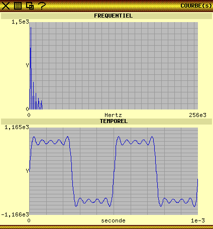
The
following screenshot gives the chart of a reverse transform of Fourier
of 512 points reconstituting a rectangular signal starting from the
fundamental frequency and the first 4 harmonics (odd):
This screenshot gives tha
reconstituting a triangular signal starting from the fundamental
fequency and the first 4 harmonics:

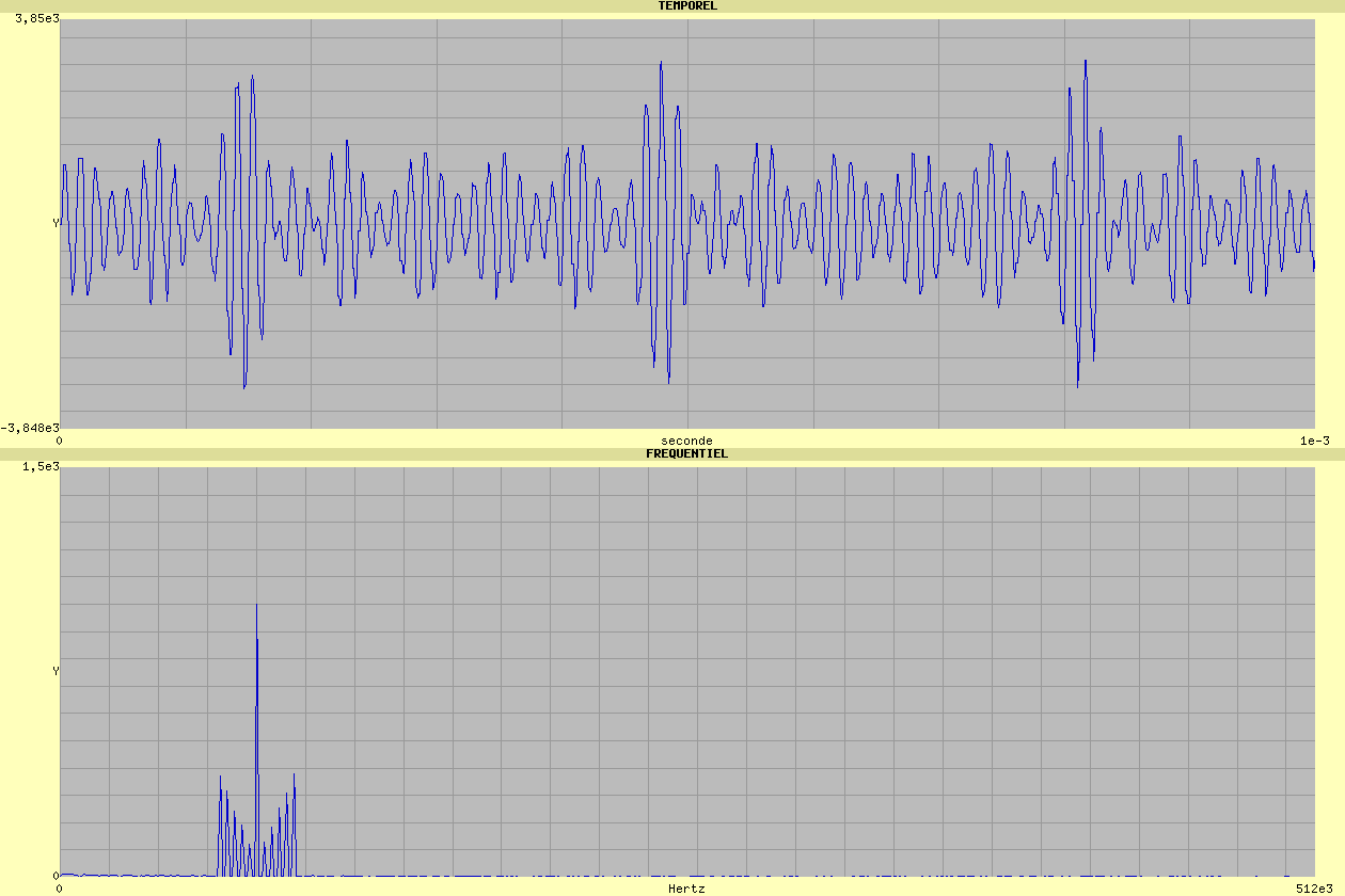
Example
Here for
example a study of several kinds of modulations using the program fft.txt file. The curves presented in this page are of 1024 dots,
the program makes it possible to also calculate them into 256,512,2048
and 4096 dots.
First of all, the modulating signal f(T) which is the sum of 5 sinus waves of 3,6,9,12 and 15 Khz:

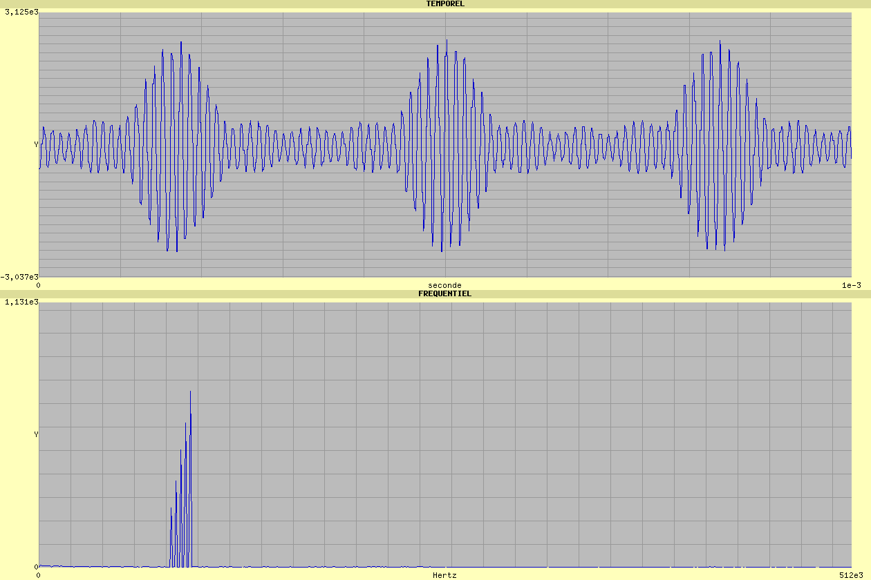
Here now carrying F(T), sinus wave of 80 Khz:

The double sideband (DSB):


The suppressed carried double sideband (DSB-SC):


And finally the single sideband (SSB):